Motivation

Data wrangling

Loading the gapminder and dplyr packages

Lade die Bibliotheken gapminder und dplyr.

# Load the gapminder package
library(gapminder)

# Load the dplyr package
library(dplyr)

# Look at the gapminder dataset
gapminder

## # A tibble: 1,704 x 6
##    country     continent  year lifeExp      pop gdpPercap
##    <fct>       <fct>     <int>   <dbl>    <int>     <dbl>
##  1 Afghanistan Asia       1952    28.8  8425333      779.
##  2 Afghanistan Asia       1957    30.3  9240934      821.
##  3 Afghanistan Asia       1962    32.0 10267083      853.
##  4 Afghanistan Asia       1967    34.0 11537966      836.
##  5 Afghanistan Asia       1972    36.1 13079460      740.
##  6 Afghanistan Asia       1977    38.4 14880372      786.
##  7 Afghanistan Asia       1982    39.9 12881816      978.
##  8 Afghanistan Asia       1987    40.8 13867957      852.
##  9 Afghanistan Asia       1992    41.7 16317921      649.
## 10 Afghanistan Asia       1997    41.8 22227415      635.
## # ... with 1,694 more rows

Understanding a data frame

Zähle die Zeilen des Datensatzes.

# How many observations (rows) are in the dataset?
nrow(gapminder)

## [1] 1704

The pipe

The filter verb

Filtering for one year

Filtere die Daten des Jahres 1957 raus.

# Filter the gapminder dataset for the year 1957
gapminder %>% filter(year==1957)

## # A tibble: 142 x 6
##    country     continent  year lifeExp      pop gdpPercap
##    <fct>       <fct>     <int>   <dbl>    <int>     <dbl>
##  1 Afghanistan Asia       1957    30.3  9240934      821.
##  2 Albania     Europe     1957    59.3  1476505     1942.
##  3 Algeria     Africa     1957    45.7 10270856     3014.
##  4 Angola      Africa     1957    32.0  4561361     3828.
##  5 Argentina   Americas   1957    64.4 19610538     6857.
##  6 Australia   Oceania    1957    70.3  9712569    10950.
##  7 Austria     Europe     1957    67.5  6965860     8843.
##  8 Bahrain     Asia       1957    53.8   138655    11636.
##  9 Bangladesh  Asia       1957    39.3 51365468      662.
## 10 Belgium     Europe     1957    69.2  8989111     9715.
## # ... with 132 more rows

Filtering for one country and one year

Erstelle zwei Filter für das Jahr 2002 und das Land China.

# Filter for China in 2002
gapminder %>% filter(country=="China",year==2002)

## # A tibble: 1 x 6
##   country continent  year lifeExp        pop gdpPercap
##   <fct>   <fct>     <int>   <dbl>      <int>     <dbl>
## 1 China   Asia       2002    72.0 1280400000     3119.

The arrange verb

Arranging observations by life expectancy

Sortiere die Daten nach Lebenserwartung. Wie sehen die Daten aus? Sortiere die Daten nochmals in absteigender Reihenfolge

# Sort in ascending order of lifeExp
gapminder %>% arrange(lifeExp)

## # A tibble: 1,704 x 6
##    country      continent  year lifeExp     pop gdpPercap
##    <fct>        <fct>     <int>   <dbl>   <int>     <dbl>
##  1 Rwanda       Africa     1992    23.6 7290203      737.
##  2 Afghanistan  Asia       1952    28.8 8425333      779.
##  3 Gambia       Africa     1952    30    284320      485.
##  4 Angola       Africa     1952    30.0 4232095     3521.
##  5 Sierra Leone Africa     1952    30.3 2143249      880.
##  6 Afghanistan  Asia       1957    30.3 9240934      821.
##  7 Cambodia     Asia       1977    31.2 6978607      525.
##  8 Mozambique   Africa     1952    31.3 6446316      469.
##  9 Sierra Leone Africa     1957    31.6 2295678     1004.
## 10 Burkina Faso Africa     1952    32.0 4469979      543.
## # ... with 1,694 more rows

# Sort in descending order of lifeExp
gapminder %>% arrange(desc(lifeExp))

## # A tibble: 1,704 x 6
##    country          continent  year lifeExp       pop gdpPercap
##    <fct>            <fct>     <int>   <dbl>     <int>     <dbl>
##  1 Japan            Asia       2007    82.6 127467972    31656.
##  2 Hong Kong, China Asia       2007    82.2   6980412    39725.
##  3 Japan            Asia       2002    82   127065841    28605.
##  4 Iceland          Europe     2007    81.8    301931    36181.
##  5 Switzerland      Europe     2007    81.7   7554661    37506.
##  6 Hong Kong, China Asia       2002    81.5   6762476    30209.
##  7 Australia        Oceania    2007    81.2  20434176    34435.
##  8 Spain            Europe     2007    80.9  40448191    28821.
##  9 Sweden           Europe     2007    80.9   9031088    33860.
## 10 Israel           Asia       2007    80.7   6426679    25523.
## # ... with 1,694 more rows

Filtering and arranging

Filtere zuerst die Daten aus 1957 raus und dann sortiere absteigend nach Bevölkerungszahl

# Filter for the year 1957, then arrange in descending order of population
gapminder %>% filter(year==1957)%>%arrange(desc(pop))

## # A tibble: 142 x 6
##    country        continent  year lifeExp       pop gdpPercap
##    <fct>          <fct>     <int>   <dbl>     <int>     <dbl>
##  1 China          Asia       1957    50.5 637408000      576.
##  2 India          Asia       1957    40.2 409000000      590.
##  3 United States  Americas   1957    69.5 171984000    14847.
##  4 Japan          Asia       1957    65.5  91563009     4318.
##  5 Indonesia      Asia       1957    39.9  90124000      859.
##  6 Germany        Europe     1957    69.1  71019069    10188.
##  7 Brazil         Americas   1957    53.3  65551171     2487.
##  8 United Kingdom Europe     1957    70.4  51430000    11283.
##  9 Bangladesh     Asia       1957    39.3  51365468      662.
## 10 Italy          Europe     1957    67.8  49182000     6249.
## # ... with 132 more rows

The mutate verb

Using mutate to change or create a column

Erstelle eine neue Variable die die Lebenserwartung in Monaten zeigt. Nenne die Variable lifeExpMonths

# Use mutate to change lifeExp to be in months
gapminder %>% mutate(lifeExp = 12 ** lifeExp)

## # A tibble: 1,704 x 6
##    country     continent  year lifeExp      pop gdpPercap
##    <fct>       <fct>     <int>   <dbl>    <int>     <dbl>
##  1 Afghanistan Asia       1952 1.21e31  8425333      779.
##  2 Afghanistan Asia       1957 5.42e32  9240934      821.
##  3 Afghanistan Asia       1962 3.39e34 10267083      853.
##  4 Afghanistan Asia       1967 5.17e36 11537966      836.
##  5 Afghanistan Asia       1972 8.82e38 13079460      740.
##  6 Afghanistan Asia       1977 3.03e41 14880372      786.
##  7 Afghanistan Asia       1982 1.02e43 12881816      978.
##  8 Afghanistan Asia       1987 1.13e44 13867957      852.
##  9 Afghanistan Asia       1992 9.41e44 16317921      649.
## 10 Afghanistan Asia       1997 1.17e45 22227415      635.
## # ... with 1,694 more rows

# Use mutate to create a new column called lifeExpMonths
gapminder %>% mutate(lifeExpMonths = 12 * lifeExp)

## # A tibble: 1,704 x 7
##    country     continent  year lifeExp      pop gdpPercap lifeExpMonths
##    <fct>       <fct>     <int>   <dbl>    <int>     <dbl>         <dbl>
##  1 Afghanistan Asia       1952    28.8  8425333      779.          346.
##  2 Afghanistan Asia       1957    30.3  9240934      821.          364.
##  3 Afghanistan Asia       1962    32.0 10267083      853.          384.
##  4 Afghanistan Asia       1967    34.0 11537966      836.          408.
##  5 Afghanistan Asia       1972    36.1 13079460      740.          433.
##  6 Afghanistan Asia       1977    38.4 14880372      786.          461.
##  7 Afghanistan Asia       1982    39.9 12881816      978.          478.
##  8 Afghanistan Asia       1987    40.8 13867957      852.          490.
##  9 Afghanistan Asia       1992    41.7 16317921      649.          500.
## 10 Afghanistan Asia       1997    41.8 22227415      635.          501.
## # ... with 1,694 more rows

Combining filter, mutate, and arrange

Kombiniere alle drei bisher gelernten Verben. Filtere zuerst das Jahr 2007 raus, leite eine neue Variable auf Monatsbasis aus der Lebenserwartung ab. und dann sortiere absteigend nach der neuen Variable.

# Filter, mutate, and arrange the gapminder dataset
gapminder %>% 
filter(year==2007) %>%
mutate(lifeExpMonths = 12 * lifeExp) %>%
arrange(desc(lifeExpMonths))

## # A tibble: 142 x 7
##    country        continent  year lifeExp      pop gdpPercap lifeExpMonths
##    <fct>          <fct>     <int>   <dbl>    <int>     <dbl>         <dbl>
##  1 Japan          Asia       2007    82.6   1.27e8    31656.          991.
##  2 Hong Kong, Ch… Asia       2007    82.2   6.98e6    39725.          986.
##  3 Iceland        Europe     2007    81.8   3.02e5    36181.          981.
##  4 Switzerland    Europe     2007    81.7   7.55e6    37506.          980.
##  5 Australia      Oceania    2007    81.2   2.04e7    34435.          975.
##  6 Spain          Europe     2007    80.9   4.04e7    28821.          971.
##  7 Sweden         Europe     2007    80.9   9.03e6    33860.          971.
##  8 Israel         Asia       2007    80.7   6.43e6    25523.          969.
##  9 France         Europe     2007    80.7   6.11e7    30470.          968.
## 10 Canada         Americas   2007    80.7   3.34e7    36319.          968.
## # ... with 132 more rows

Data visualization

Variable assignment

lade das Paket ggplot2. Filtere die Daten aus dem Jahr 1952 und speichere das in einen neuen Datensatz gapminder_1952

# Load the ggplot2 package as well
library(ggplot2)

# Create gapminder_1952
gapminder_1952 <- gapminder %>% filter(year==1952)

Comparing population and GDP per capita

Nimm den neuen Datensatz und mache eine Punktgrafik mit gdpPercap auf der x-Achse und lifeExp auf der y-Achse. Tausche auf der x-Achse gdpPercap mit pop und auf der y-Achse lifeExp mit gdpPercap aus.

gapminder_1952 <- gapminder %>%
  filter(year == 1952)

# Change to put pop on the x-axis and gdpPercap on the y-axis
ggplot(gapminder_1952, aes(x = gdpPercap, y = lifeExp)) +
  geom_point()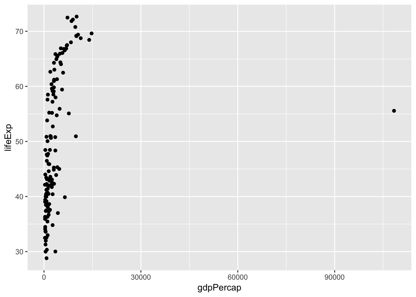

ggplot(gapminder_1952, aes(x = pop, y = gdpPercap)) +
  geom_point()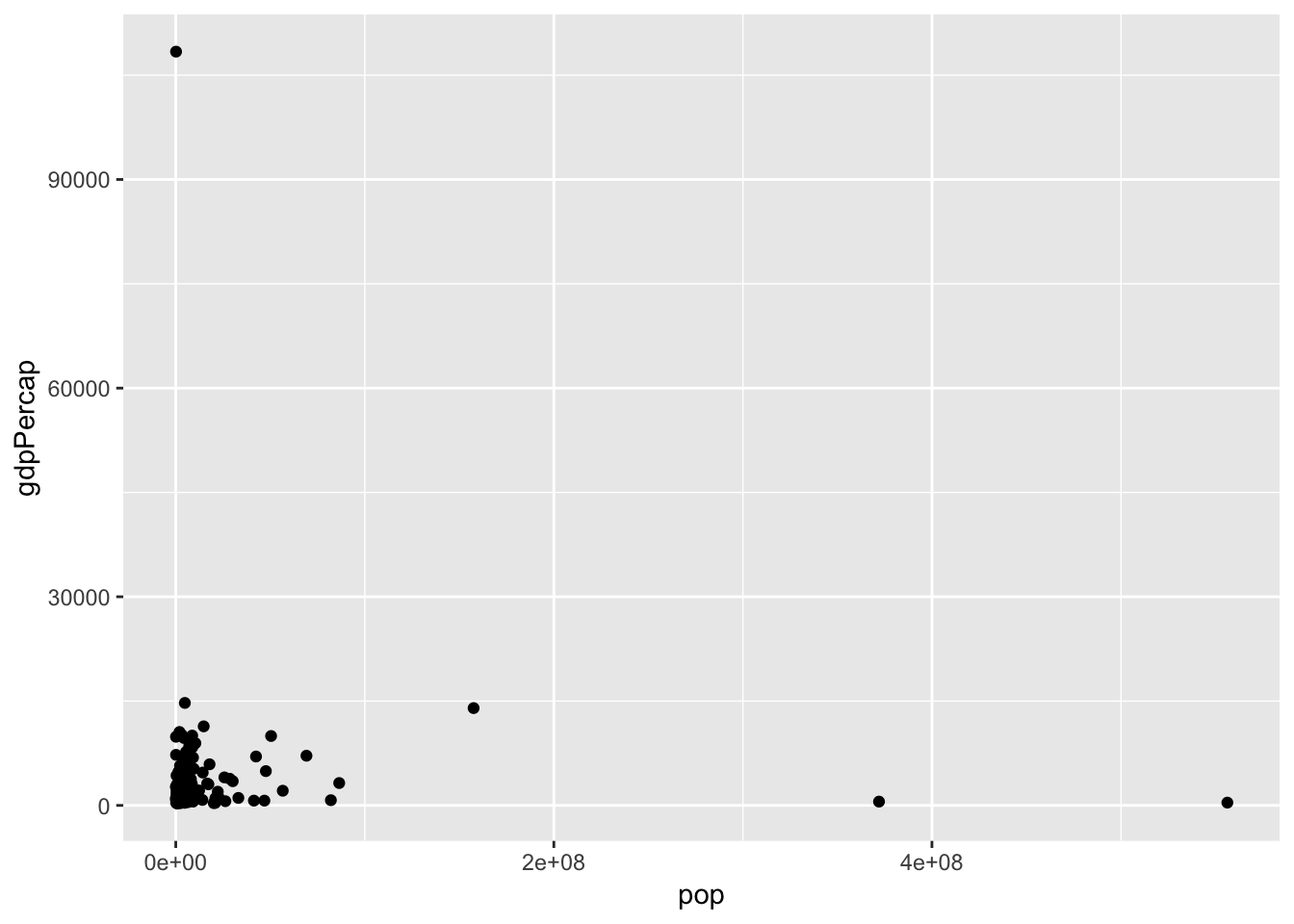

Comparing population and life expectancy

Mach die selbe Grafik mit pop und lifeExp

gapminder_1952 <- gapminder %>%
  filter(year == 1952)

# Create a scatter plot with pop on the x-axis and lifeExp on the y-axis
ggplot(gapminder_1952, aes(x = pop, y = lifeExp)) +
  geom_point()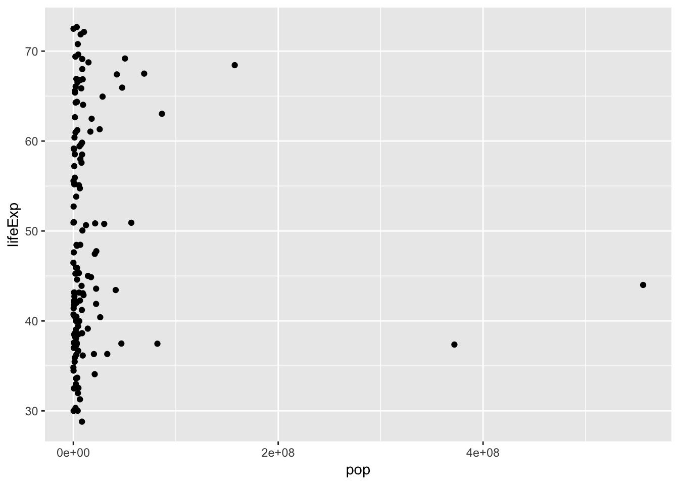

Log Scales

Putting the x-axis on a log scale

Logarithmiere die x-Achse. Wird die Grafik dadurch besser?

gapminder_1952 <- gapminder %>%
  filter(year == 1952)

# Change this plot to put the x-axis on a log scale
ggplot(gapminder_1952, aes(x = pop, y = lifeExp)) +
  geom_point()+scale_x_log10()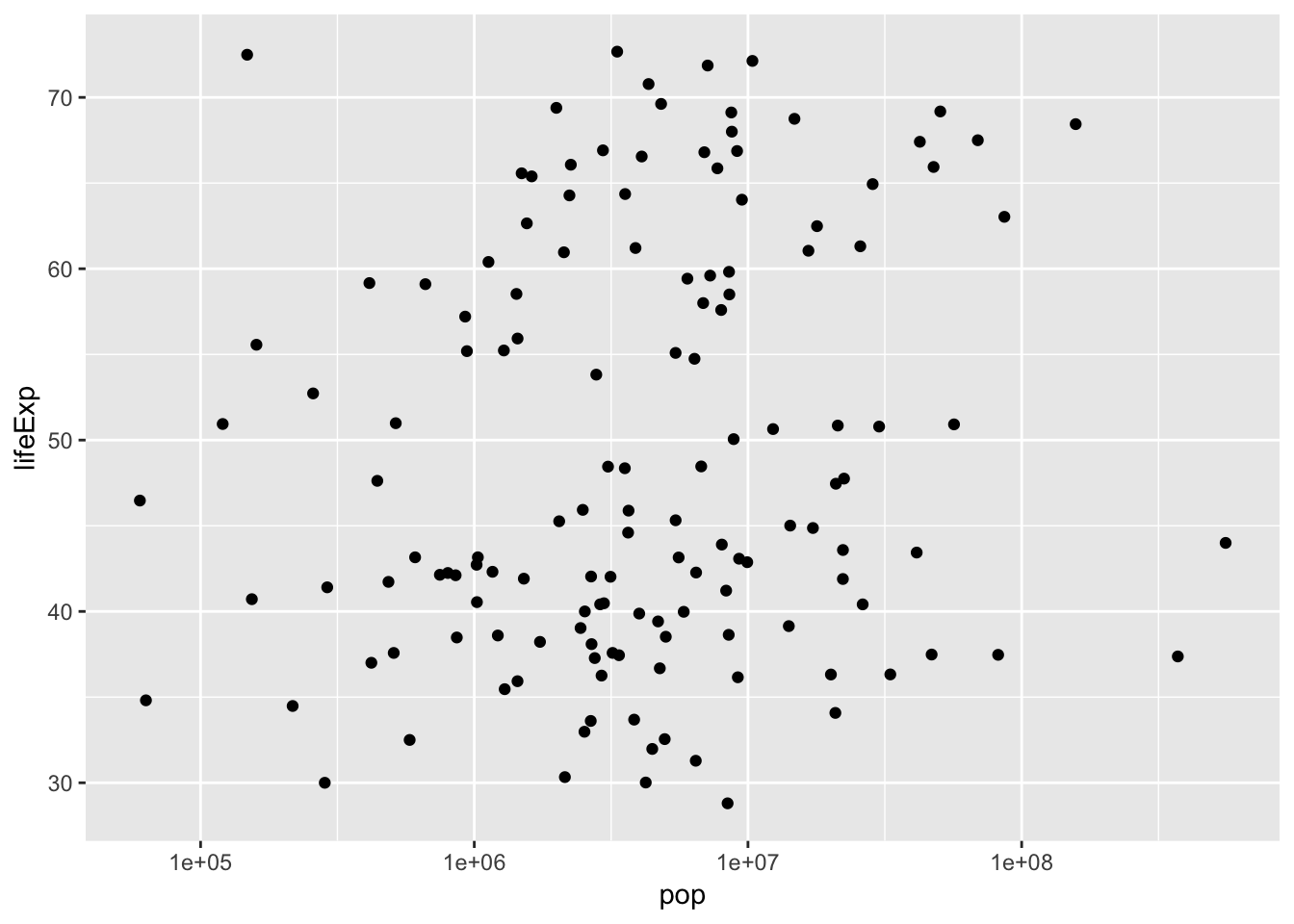

Putting the x- and y- axes on a log scale

Logarithmiere beide Achsen.

gapminder_1952 <- gapminder %>%
  filter(year == 1952)

# Scatter plot comparing pop and gdpPercap, with both axes on a log scale
ggplot(gapminder_1952, aes(x = pop, y = gdpPercap)) +
  geom_point()+scale_x_log10() +
  scale_y_log10()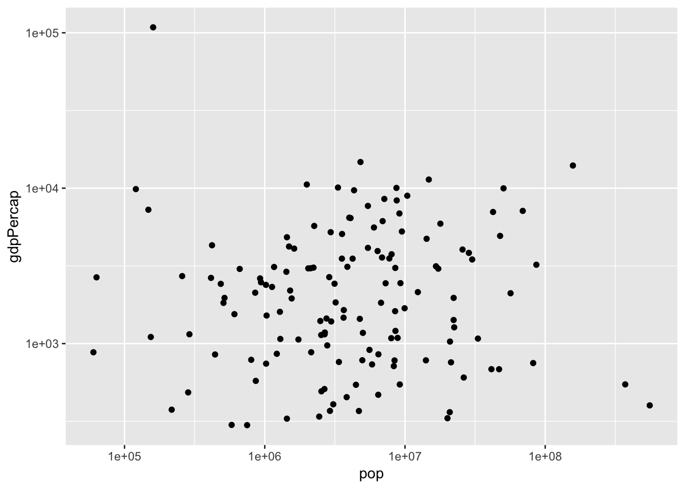

Adding color to a scatter plot

Füge eine dritte ästhetische Komponente hinzu. Färbe die Grafik nach Kontinenten ein.

gapminder_1952 <- gapminder %>%
  filter(year == 1952)

# Scatter plot comparing pop and lifeExp, with color representing continent
ggplot(gapminder_1952, aes(x = pop, y = lifeExp,color=continent)) +
  geom_point()+scale_x_log10() +
  scale_y_log10()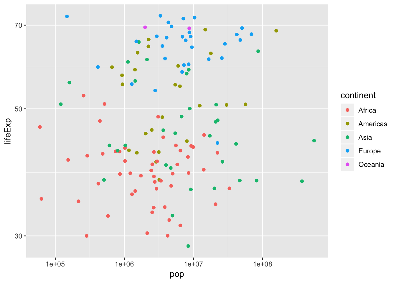

Adding size and color to a plot

Füge eine vierte ästhetische Komponente hinzu. Mache die Punktgröße vom gdpPercap abhängig.

gapminder_1952 <- gapminder %>%
  filter(year == 1952)

# Add the size aesthetic to represent a country's gdpPercap
ggplot(gapminder_1952, aes(x = pop, y = lifeExp, color = continent,size=gdpPercap)) +
  geom_point() +
  scale_x_log10()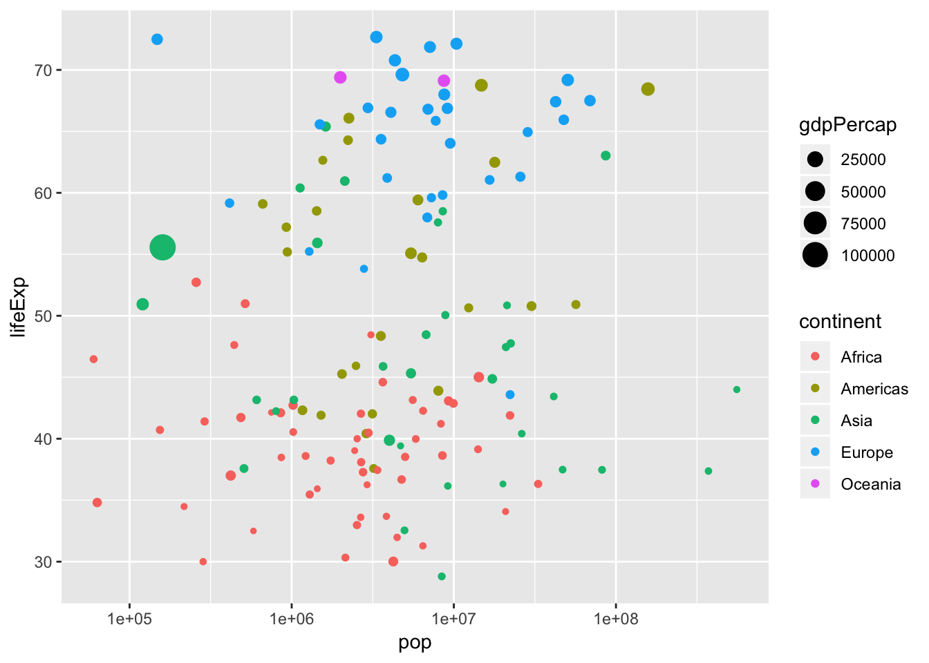

Faceting

Creating a subgraph for each continent

Separiere die Grafik in Facetten für jeden Kontinent.

gapminder_1952 <- gapminder %>%
  filter(year == 1952)

# Scatter plot comparing pop and lifeExp, faceted by continent
ggplot(gapminder_1952, aes(x = pop, y = lifeExp)) +
  geom_point() +
  scale_x_log10()+
  facet_wrap(~ continent)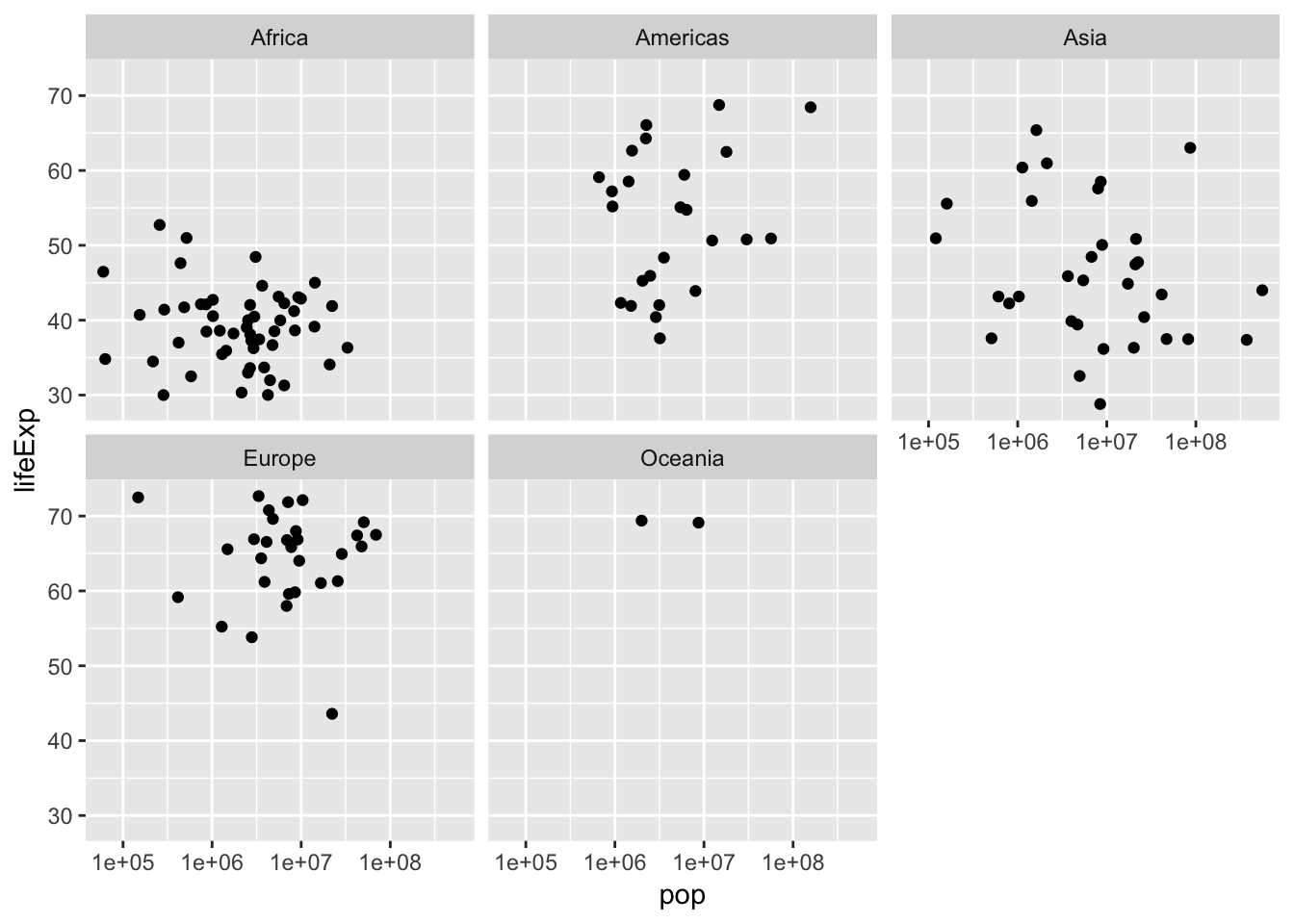

Faceting by year

Separiere die Grafik in Facetten für jedes Jahr.

# Scatter plot comparing gdpPercap and lifeExp, with color representing continent
# and size representing population, faceted by year
ggplot(gapminder, aes(x = gdpPercap, y = lifeExp,color=continent,size=pop)) +
  geom_point() +
  scale_x_log10()+
  facet_wrap(~ year)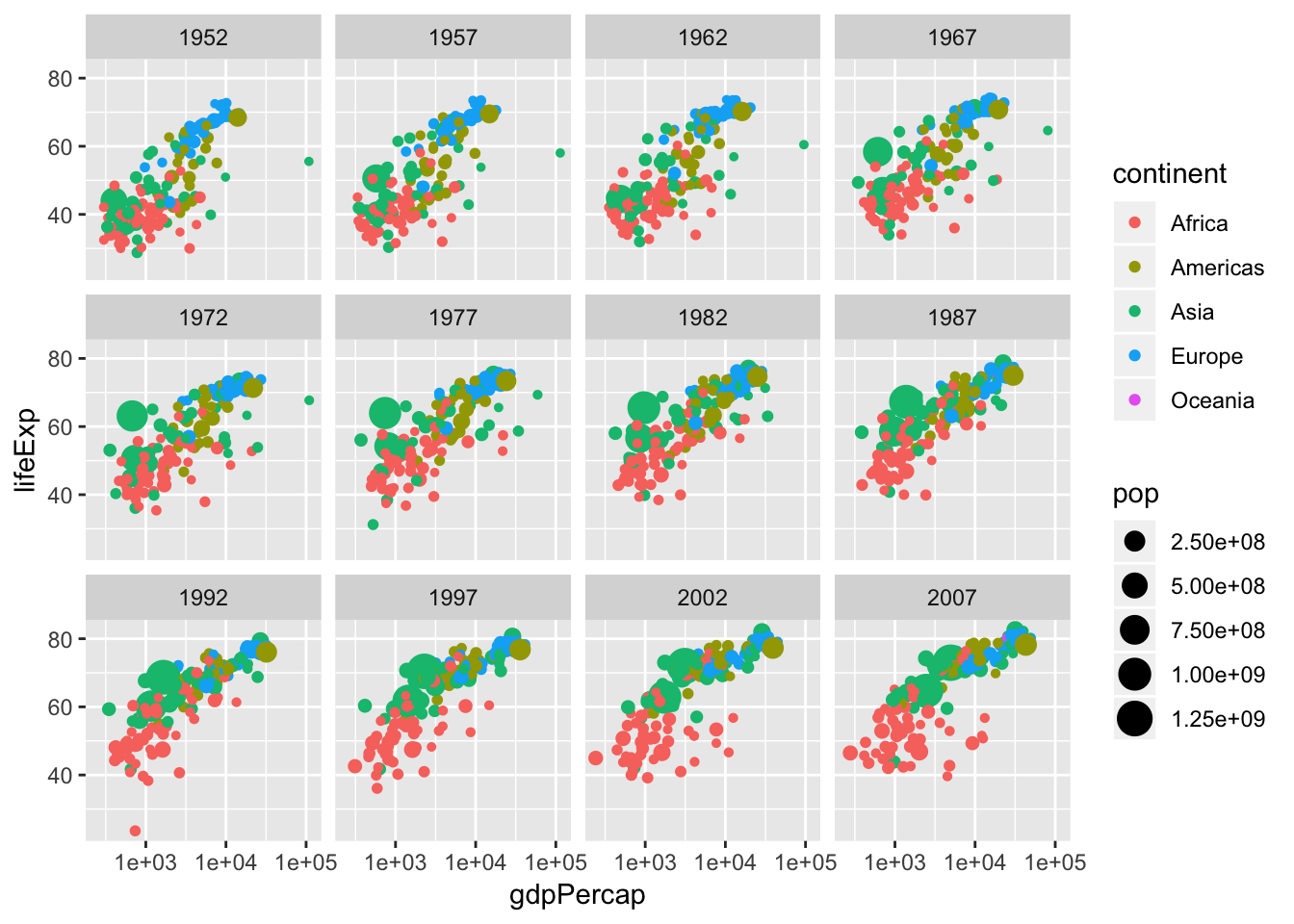

Endgegner

# install.packages('devtools')
#devtools::install_github('thomasp85/gganimate')

library(gapminder)
library(gganimate)

ggplot(gapminder, aes(gdpPercap, lifeExp, size = pop, colour = country)) +
  geom_point(alpha = 0.7, show.legend = FALSE) +
  scale_colour_manual(values = country_colors) +
  scale_size(range = c(2, 12)) +
  scale_x_log10() +
  facet_wrap(~continent) +
  # Here comes the gganimate specific bits
  labs(title = 'Year: {frame_time}', x = 'GDP per capita', y = 'life expectancy') +
  transition_time(year) +
  ease_aes('linear')

Grouping and summarizing

Summarizing the median life expectancy

# Summarize to find the median life expectancy
gapminder %>% summarise(medianLifeExp = median(lifeExp))

## # A tibble: 1 x 1
##   medianLifeExp
##           <dbl>
## 1          60.7

Summarizing the median life expectancy in 1957

# Filter for 1957 then summarize the median life expectancy
gapminder %>% 
filter(year==1957) %>%
summarise(medianLifeExp = median(lifeExp))

## # A tibble: 1 x 1
##   medianLifeExp
##           <dbl>
## 1          48.4

Summarizing multiple variables in 1957

# Filter for 1957 then summarize the median life expectancy and the maximum GDP per capita
gapminder %>% 
filter(year == 1957) %>%
summarise(medianLifeExp = median(lifeExp),
      maxGdpPercap = max(gdpPercap))

## # A tibble: 1 x 2
##   medianLifeExp maxGdpPercap
##           <dbl>        <dbl>
## 1          48.4      113523.

group_by verb

Summarizing by year

# Find median life expectancy and maximum GDP per capita in each year

gapminder %>% 
group_by(year) %>%
summarise(medianLifeExp = median(lifeExp),
      maxGdpPercap = max(gdpPercap))

## # A tibble: 12 x 3
##     year medianLifeExp maxGdpPercap
##    <int>         <dbl>        <dbl>
##  1  1952          45.1      108382.
##  2  1957          48.4      113523.
##  3  1962          50.9       95458.
##  4  1967          53.8       80895.
##  5  1972          56.5      109348.
##  6  1977          59.7       59265.
##  7  1982          62.4       33693.
##  8  1987          65.8       31541.
##  9  1992          67.7       34933.
## 10  1997          69.4       41283.
## 11  2002          70.8       44684.
## 12  2007          71.9       49357.

Summarizing by continent

# Find median life expectancy and maximum GDP per capita in each continent in 1957

gapminder %>% 
filter(year == 1957) %>%
group_by(continent) %>%
summarise(medianLifeExp = median(lifeExp),
      maxGdpPercap = max(gdpPercap))

## # A tibble: 5 x 3
##   continent medianLifeExp maxGdpPercap
##   <fct>             <dbl>        <dbl>
## 1 Africa             40.6        5487.
## 2 Americas           56.1       14847.
## 3 Asia               48.3      113523.
## 4 Europe             67.6       17909.
## 5 Oceania            70.3       12247.

Summarizing by continent and year

# Find median life expectancy and maximum GDP per capita in each year/continent combination
gapminder %>% 
group_by(continent,year) %>%
summarise(medianLifeExp = median(lifeExp),
      maxGdpPercap = max(gdpPercap))

## # A tibble: 60 x 4
## # Groups:   continent [?]
##    continent  year medianLifeExp maxGdpPercap
##    <fct>     <int>         <dbl>        <dbl>
##  1 Africa     1952          38.8        4725.
##  2 Africa     1957          40.6        5487.
##  3 Africa     1962          42.6        6757.
##  4 Africa     1967          44.7       18773.
##  5 Africa     1972          47.0       21011.
##  6 Africa     1977          49.3       21951.
##  7 Africa     1982          50.8       17364.
##  8 Africa     1987          51.6       11864.
##  9 Africa     1992          52.4       13522.
## 10 Africa     1997          52.8       14723.
## # ... with 50 more rows

Visualizing summarized data

Visualizing median life expectancy over time

by_year <- gapminder %>%
  group_by(year) %>%
  summarize(medianLifeExp = median(lifeExp),
            maxGdpPercap = max(gdpPercap))

# Create a scatter plot showing the change in medianLifeExp over time
by_year %>% 
ggplot(aes(x=year,y=medianLifeExp))+
geom_point()+expand_limits(y = 0)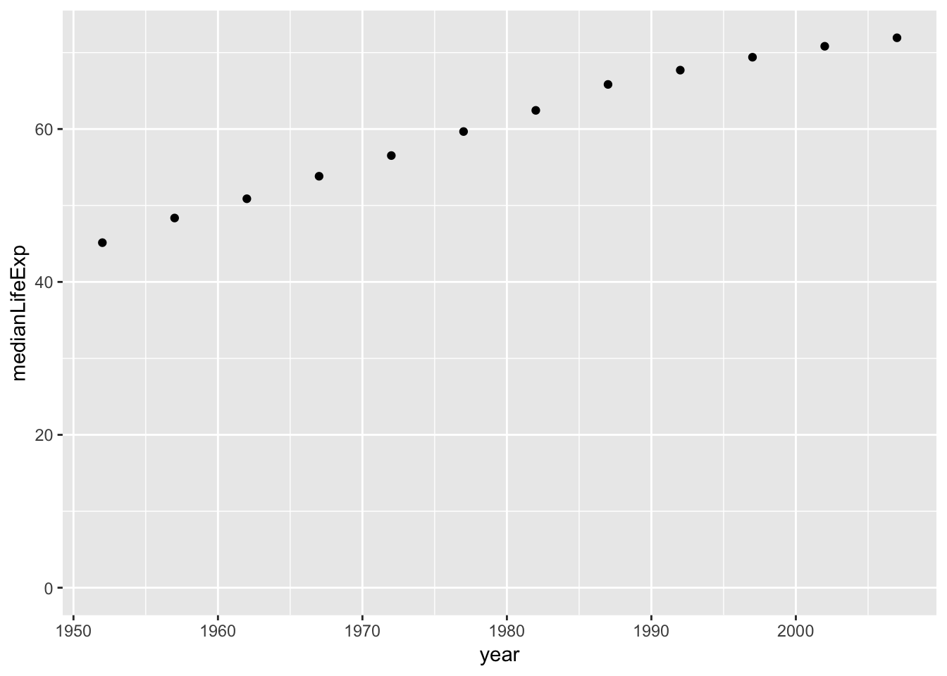

Visualizing median GDP per capita per continent over time

# Summarize medianGdpPercap within each continent within each year: by_year_continent
by_year_continent <- gapminder %>%
  group_by(continent, year) %>%
  summarize(medianGdpPercap = median(gdpPercap))

# Plot the change in medianGdpPercap in each continent over time
by_year_continent %>% 
ggplot(aes(x=year,y=medianGdpPercap,color=continent))+
geom_point()+expand_limits(y = 0)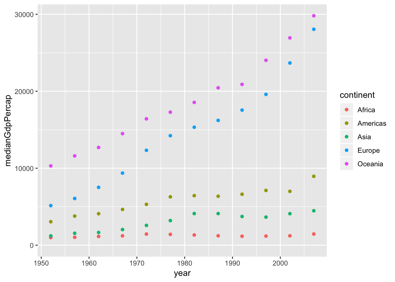

Comparing median life expectancy and median GDP per continent in 2007

# Summarize the median GDP and median life expectancy per continent in 2007
by_continent_2007 <- gapminder %>%
  filter(year == 2007) %>%
  group_by(continent) %>% 
  summarize(medianLifeExp = median(lifeExp), 
  medianGdpPercap = median(gdpPercap))


# Use a scatter plot to compare the median GDP and median life expectancy
by_continent_2007 %>% 
ggplot(aes(x=medianGdpPercap,y=medianLifeExp,color=continent))+
geom_point()+expand_limits(y = 0)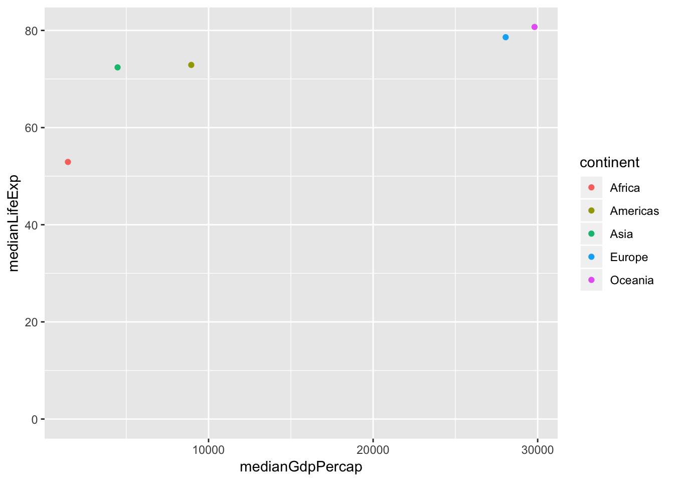

Types of visualizations

Line plots

Visualizing median GDP per capita over time

# Summarize the median gdpPercap by year, then save it as by_year
by_year <- gapminder %>%
group_by(year)%>%
summarise(medianGdpPercap = median(gdpPercap))

# Create a line plot showing the change in medianGdpPercap over time
by_year %>% 
ggplot(aes(x=year,y=medianGdpPercap))+
geom_line()+expand_limits(y = 0)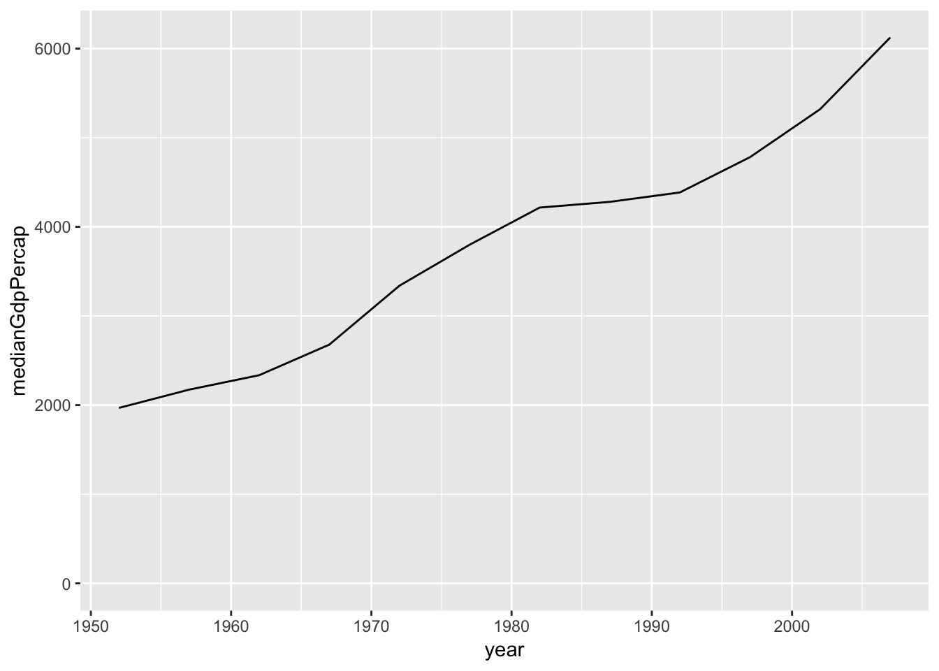

Visualizing median GDP per capita by continent over time

# Summarize the median gdpPercap by year & continent, save as by_year_continent
by_year_continent <- gapminder %>%
group_by(continent, year)%>%
summarise(medianGdpPercap = median(gdpPercap))

# Create a line plot showing the change in medianGdpPercap by continent over time
by_year_continent %>% 
ggplot(aes(x=year,y=medianGdpPercap,color=continent))+
geom_line()+expand_limits(y = 0)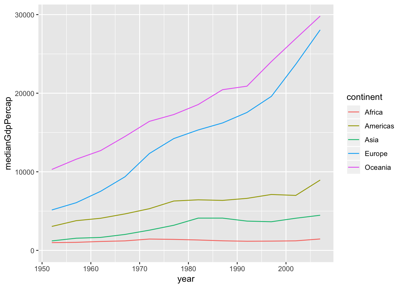

Bar Plots

Visualizing median GDP per capita by continent

# Summarize the median gdpPercap by year and continent in 1952
by_continent<- gapminder %>%
filter(year==1952) %>%
group_by(continent) %>%
summarise(medianGdpPercap = median(gdpPercap))


# Create a bar plot showing medianGdp by continent
by_continent %>% 
ggplot(aes(x=continent,y=medianGdpPercap))+
geom_col()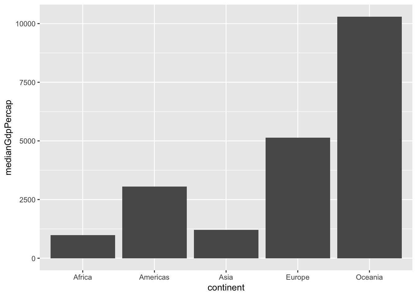

Visualizing GDP per capita by country in Oceania

# Filter for observations in the Oceania continent in 1952
oceania_1952<- gapminder %>%
filter(continent=="Oceania",year==1952)

# Create a bar plot of gdpPercap by country
oceania_1952 %>% 
ggplot(aes(x=country,y=gdpPercap))+
geom_col()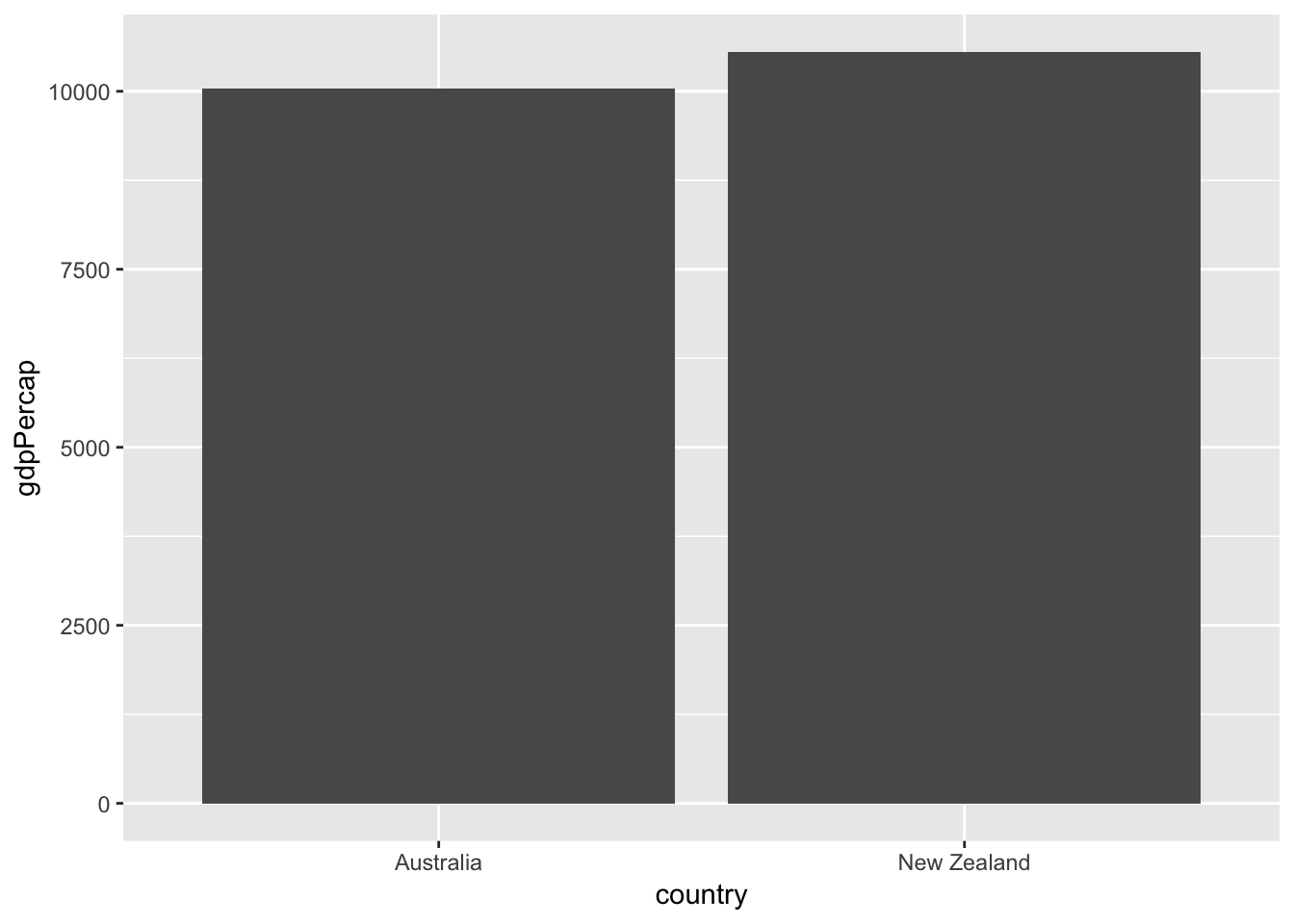

Histograms

Visualizing population

gapminder_1952 <- gapminder %>%
  filter(year == 1952)

# Create a histogram of population (pop)
gapminder_1952 %>% 
ggplot(aes(x=pop))+
geom_histogram()

## `stat_bin()` using `bins = 30`. Pick better value with `binwidth`.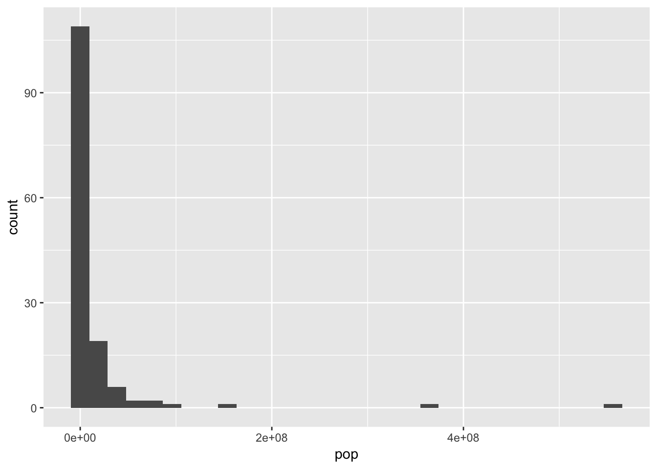

Visualizing population with x-axis on a log scale

gapminder_1952 <- gapminder %>%
  filter(year == 1952)

# Create a histogram of population (pop), with x on a log scale
gapminder_1952 %>% 
ggplot(aes(x=pop))+
geom_histogram()+
scale_x_log10()

## `stat_bin()` using `bins = 30`. Pick better value with `binwidth`.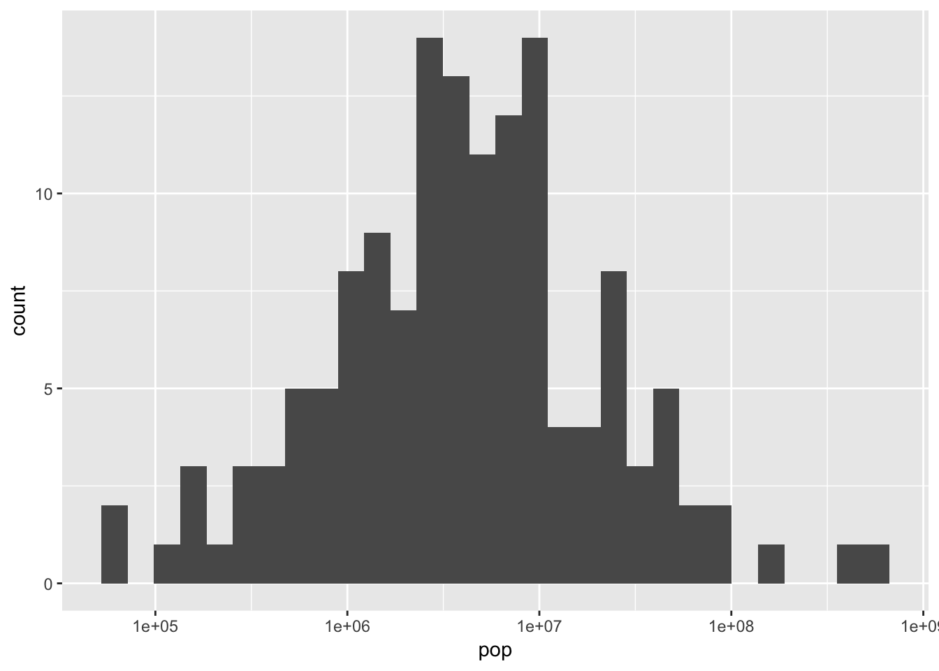

Box Plots

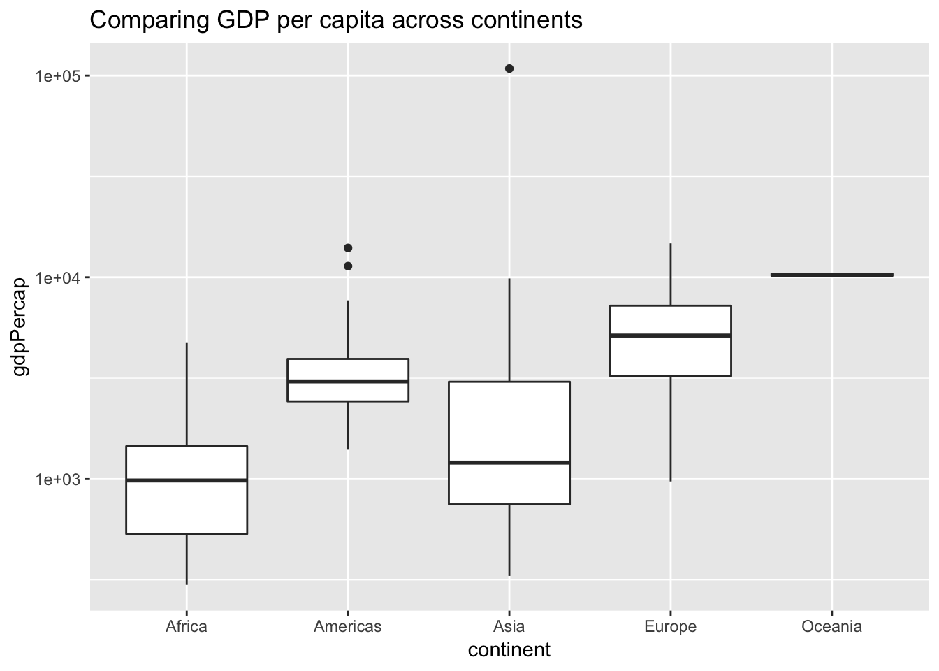
Comparing GDP per capita across continents

gapminder_1952 <- gapminder %>%
  filter(year == 1952)

# Create a boxplot comparing gdpPercap among continents
gapminder_1952 %>% 
ggplot(aes(x=continent,y=gdpPercap))+
geom_boxplot()+
scale_y_log10()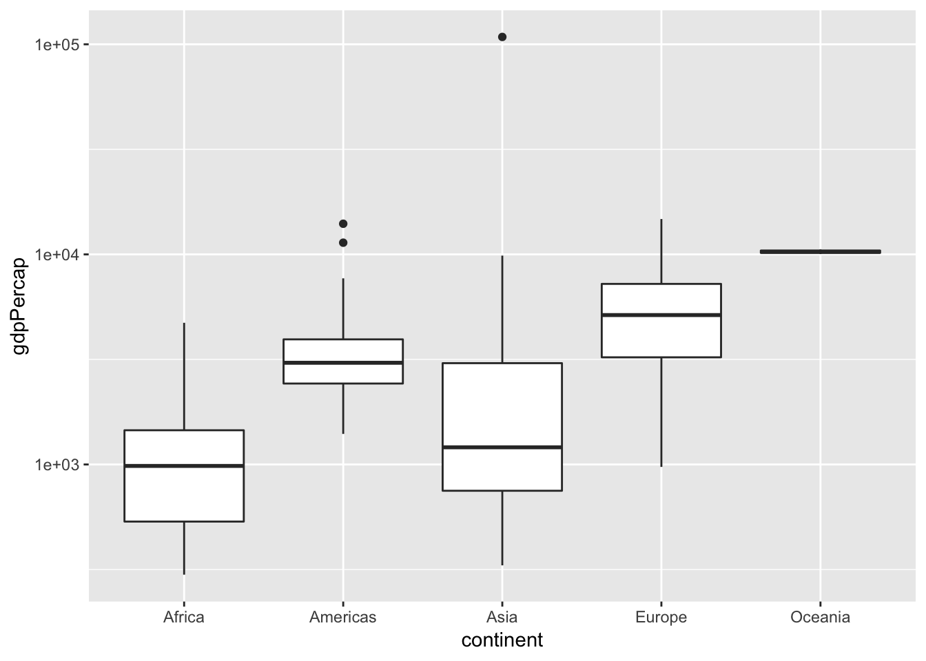

Adding a title to your graph

gapminder_1952 <- gapminder %>%
  filter(year == 1952)

# Add a title to this graph: "Comparing GDP per capita across continents"
ggplot(gapminder_1952, aes(x = continent, y = gdpPercap)) +
  geom_boxplot() +
  scale_y_log10()+
  ggtitle("Comparing GDP per capita across continents")